exploring econometrics
- Joely To

- May 25, 2020
- 3 min read
This week, my friend Mitra Stainsbury (Year 12) reveals another fascinating application of mathematics - and she's provided a fantastic list of resources at the end to deepen your understanding and interest!

What makes the business world tick on? Maths.
Econometrics, or Mathematical Economics, is the application of statistical methods to evaluate and produce economic models and economic forecasting. Without maths, economic theory becomes increasingly difficult to actually apply to real world situations, quickly leading to the misallocation of resources.
A model in economics is similar to hypothesis in science; it is proposed and then tested. The main way that econometricians can establish and quantify the relationship – a model – between two variables as well as forecasting new observations is by using a Simple Linear Regression. Here is a brief introduction as to how this is derived:
Dependent Variable – the variable whose values we want to explain or forecast – y Independent Variable – the variable that explains the existence of the dependent variable – x
1. A Simple Linear Regression is just that – linear. The formula used in econometrics is the exactly same as our formula for a straight-line graph, just with Greek letter notation instead: y = mx + c is equivalent to y = β0 + β1x , where: β0 = y-intercept/constant and β1 = gradient/slope.

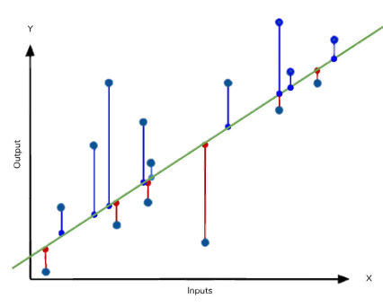
2. Unfortunately, data is rarely perfectly linear! As we see in scatter graphs, there is often a general trend but the majority of these data points will deviate marginally from the overall trend. These distances away from the trend line are called residuals. The total value of positive residuals always sums with the total value of negative residuals to equal zero because the trend line is the average of the two, the ‘best fit’. This means that the distance from each point to the best fit line is minimised which is known as the error term.
Therefore, we have to include this in our equation:
y = β0 + β1x + ε , where: ε is the error term (which is non-constant)
3. Now all we need to do is apply the equation to the model that is being tested; for example: ‘Income explains consumption’
Dependent variable = Consumption Independent variable = Income
Consumption = β0 + β1Income + ε Using data provided for both variables, the value of β0 and β1 can be calculated using a least-squares solution. (see appendix)
Econometrics is a great tool firms use to advise their managerial decisions on a micro scale as well as for government policy making on a macro scale. Despite this, the economy is always unpredictable and whilst we may do our best to use econometrics as a keyhole into its intricacies, the results are at best a guess and not a guarantee. In the words of the economist John Kenneth Galbraith, ‘economic forecasting [makes] astrology look respectable’, so always take it with a pinch of salt!
Appendix:
If this has sparked your interest then here are some resources for you to continue your journey in exploring Econometrics:
https://www.youtube.com/watch?v=owI7zxCqNY0 – this video talks through the concepts discussed in this article and walks through the example of ‘income explains consumption’
https://www.albert.io/econometrics - have a go at some questions yourself!
https://www.youtube.com/watch?v=ZkjP5RJLQF4&list=PLIeGtxpvyG-LoKUpV0fSY8BGKIMIdmfCi&index=1 – this is the first in a series of videos explaining Simple Linear Regression in detail, including how to calculate the error term and use least-squares solutions – recommended for Further Maths statisticians
https://www.research-live.com/article/opinion/econometrics-an-able-servant-but-never-the-master/id/4009208 - an interesting article furthering the discussion of to what extent we should rely on econometrics and the models they produce
Bibliography
Image showing error on a regression graph, Dataquest, accessed 3 May 2020, <https://www.dataquest.io/blog/understanding-regression-error-metrics/>


Comments